
dbt (data build tool) helps analytics teams transform data directly inside modern cloud warehouses. It brings software engineering best practices such as version control, testing and documentation to SQL-based analytics. Teams widely adopt dbt because it creates reliable, testable and well-documented data pipelines. The tool supports Snowflake, BigQuery, Databricks, Redshift and several other platforms.
Two core concepts models and macros form the foundation of almost every dbt project. Both use SQL files combined with Jinja templating syntax. Despite surface similarities, their purposes and behaviors differ significantly. Understanding this distinction prevents code duplication and improves long-term project quality.
Why Clear Separation Between Models and Macros Matters
Many beginners mix model logic with macro logic, creating hard-to-maintain projects. Clean separation follows the single-responsibility principle known from software design. Models focus on business transformation outcomes. Macros handle reusable SQL generation patterns. When responsibilities blur, small changes ripple across dozens of files.
Teams waste time hunting repeated code blocks during refactors. Proper usage leads to faster onboarding for new team members. It also makes testing and debugging more predictable. Clear boundaries scale better as project size grows from dozens to thousands of models.
What dbt Models Really Represent in Practice
A dbt model is essentially a SQL SELECT statement wrapped in a .sql file. That statement defines exactly what data should exist after transformation. Models live inside the models/ directory with meaningful subfolder organization. When executed, dbt turns the SELECT into a real database object. Common materializations include full tables, lightweight views and efficient incremental tables.
Ephemeral materialization keeps logic as a CTE without creating objects. Every model contributes one clear step in the overall transformation DAG. The directed acyclic graph automatically determines correct execution order. Models therefore represent the “what” part of analytics engineering work.
How Models Appear in the dbt Workflow
You typically run dbt run to build all models or dbt run –select specific_model to target one file. dbt compiles Jinja first, then executes the resulting SQL against your warehouse. Dependencies declared with {{ ref(‘upstream_model’) }} ensure correct sequencing. Sources declared with {{ source(‘raw’, ‘orders’) }} point to external tables. Models integrate tightly with YAML-based testing and documentation features. Column-level tests catch data quality issues early. Table-level tests verify business rules. Documentation appears automatically in the generated dbt docs site. Models therefore form the visible, queryable assets that analysts and BI tools consume daily.
Typical Folder Structure Used for Models
Most mature projects organize models into three conceptual layers. Staging models clean and lightly rename raw source data. Intermediate models perform joins, filters and business-specific calculations. Marts models deliver clean, wide, denormalized tables ready for reporting. Some teams add an intermediate analytics layer for complex metrics. Folder names usually reflect these layers staging/, intermediate/, marts/. Consistent naming conventions help team members quickly understand purpose. Subfolders inside each layer group related concepts together logically. Good structure reduces cognitive load during debugging sessions.
Materialization Types That Models Support
The most common materialization remains table dbt drops and recreates the full object each run. View materialization creates no physical storage and stays lightweight. Incremental materialization appends or merges only new or changed records. Ephemeral materialization inlines the logic as a CTE inside dependent models. Incremental models dramatically reduce warehouse costs on large historical datasets. Each materialization type suits different performance and freshness requirements. Teams often configure materialization globally in dbt_project.yml then override per model when needed. Choosing the right type becomes an important cost-control decision.
Core Purpose of dbt Macros Explained Simply
Macros serve as reusable Jinja + SQL code blocks inside dbt projects. They behave similarly to functions in conventional programming languages. Macros generate SQL fragments during the compilation phase only. Unlike models, macros never create tables or views themselves. Their entire job finishes before any warehouse query actually executes. Developers place macro definitions inside the macros/ directory. Calling syntax uses double curly braces like normal Jinja expressions. Macros therefore represent the “how” part of consistent SQL generation patterns.
Where Macros Live and How They Get Named
Macro files end with .sql extension just like model files. File names should describe the macro’s single responsibility clearly. Popular examples include format_date.sql, cents_to_dollars.sql or generate_schema_name.sql. Many teams create a utils/ subfolder inside macros/ for general-purpose helpers. Other subfolders might hold macros specific to finance, marketing or slowly changing dimensions. Consistent naming reduces time spent searching documentation. Descriptive names also serve as self-documentation during code reviews. Good naming becomes especially valuable as macro count grows.
The dbt Compilation Phase Where Macros Execute
dbt processes projects in distinct phases during every command. Parsing reads all .sql files and YAML configurations first. It builds an internal manifest containing resources and dependencies. Compilation then renders every Jinja expression present in the project. Macro calls expand fully during this rendering step. The final plain SQL output lands inside the target/compiled/ folder. Execution phase only begins after successful compilation completes. Macros therefore never reach the warehouse execution engine directly. This compile-time nature gives macros tremendous flexibility.
Basic Macro Syntax and Parameter Usage
Every macro starts with {% macro name(param1, param2=default) %}. Logic lives between the opening and {% endmacro %} tags. Parameters accept default values for optional behavior. Inside the macro body you mix plain SQL with Jinja control structures. Calling syntax remains {{ macro_name(arg1, arg2) }} almost everywhere. Arguments can be strings, numbers, booleans or even other macro results. Macros frequently return formatted strings using the {{ return(value) }} helper. Clean parameter design prevents confusing calls in downstream models.
Practical Example Simple Cents to Dollars Macro
Many e-commerce datasets store money values in integer cents columns. Repeated division by 100 appears in dozens of models. A small macro centralizes this pattern safely.
jinja
{% macro cents_to_dollars(amount_column, decimals=2) %}
round( {{ amount_column }} / 100.0, {{ decimals }} )
{% endmacro %}
Usage becomes {{ cents_to_dollars(‘order_total_cents’) }} as order_total. One-line change updates rounding behavior everywhere instantly. Default parameter allows override when business rules differ. Small utility macros like this appear in nearly every serious dbt project.
More Advanced Example Date Spine Macro Pattern
Time-series analysis frequently requires complete date ranges without gaps. Writing UNION ALL statements manually grows tedious quickly. A date spine macro solves this problem elegantly.
jinja
{% macro get_date_spine(datepart, start_date, end_date) %}
{{ return(adapter.dispatch(‘get_date_spine’, ‘my_macros’)(datepart, start_date, end_date)) }}
{% endmacro %}
The dispatched implementation usually uses a large numbers table or recursive CTE. One macro call generates thousands of date rows reliably. Dispatch mechanism allows database-specific optimizations when necessary. Teams reuse this macro across dozens of calendar and metric models.
Comparison Table Purpose and Responsibilities
Models exist to produce final transformed datasets inside the warehouse. Macros exist purely to generate correct SQL text during compilation. Models always materialize something tangible. Macros materialize nothing themselves. Models participate actively in the dbt DAG structure. Macros remain invisible in lineage graphs. Models support native tests on columns and tables. Macros cannot have tests applied directly. Models appear prominently in generated documentation sites. Macros stay hidden utility functions. This sharp division guides correct usage decisions.
Comparison Table Execution Timing Differences
dbt executes models during the runtime phase after compilation finishes. Macro logic runs entirely during the earlier compilation phase. Model SQL reaches the warehouse and processes actual data rows. Macro SQL never executes as standalone queries. Model execution consumes warehouse compute credits directly. Macro expansion consumes only local dbt process resources. Timing difference explains why macros can influence model SQL structure dynamically. Understanding this boundary prevents many common debugging surprises.
When to Extract Logic Into a Macro Instead of Inline
Duplicate code blocks longer than about ten lines deserve macro extraction. Conditional logic depending on target name or variables belongs in macros. Loops that generate dynamic columns or CASE statements justify macros. Warehouse-specific SQL patterns should live inside dispatched macros. Business rules applied identically across multiple models warrant centralization. One-off expressions that appear only once stay inside models safely. Extraction threshold depends somewhat on team conventions and project size.
Benefits of Using Macros for Maintainability
Centralized macros reduce places where the same logic must be updated. Single change propagates everywhere the macro gets called automatically. Refactoring effort drops dramatically on large projects. Code reviews become easier when patterns use descriptive macro names. Onboarding speed improves because common utilities already exist. Testing coverage increases indirectly because macros simplify model SQL. Overall project readability rises noticeably with thoughtful macro usage.
Risks and Common Mistakes When Overusing Macros
Over-abstraction creates macros that become hard to understand quickly. Deep macro nesting hides business meaning from readers. Excessive parameters make calling syntax confusing and error-prone. Macros that query metadata during compilation can slow down every run. Poorly documented macros force developers to read implementation instead of interface. Teams sometimes create god-macros containing unrelated responsibilities. Balance remains important macros should simplify, not complicate.
Recommended Best Practices for Macro Design
Keep each macro focused on exactly one clear responsibility. Use descriptive names that reveal intent immediately. Provide sensible default parameter values whenever possible. Add inline comments explaining non-obvious decisions. Handle edge cases and null inputs gracefully inside logic. Prefer adapter.dispatch() for cross-warehouse compatibility. Group related macros together in logical subfolders. Review macro calls during model pull requests consistently. Follow these habits to keep macros valuable long-term assets.
Final Summary Models and Macros Together
Models answer the question “what final data shape do we need?”. Macros answer “how can we generate that SQL consistently?”. Models create the actual tables and views analysts query every day. Macros enable clean, DRY, maintainable transformation code. Both pieces work together to produce trustworthy analytics outputs. Mastering their distinct roles separates average dbt projects from excellent ones. Teams that respect this boundary usually deliver faster and with higher quality.